
Given a cat or dog image, determine if the image is either a cat or a dog.
The scenario is framed as a binary classification problem between a cat and a dog.
I will use a Convolutional Neural Network and Transfer Learning to create an application. I will use AWS SageMaker to prepare the Jupyter Notebooks, provision compute, and store the images in s3.
My implementation deployed both in AWS SageMaker Studio Notebook and through AWS SageMaker Script Mode.
The advantage of AWS SageMaker Script Mode is that you can run scripts without fear of being interrupted by the browser. For example, your organization might implement an 8-hour session limit in AWS SageMaker Studio to save costs from idle sessions.
The origin of CNN was first introduced by Kunihiko Fukushima in the Paper, Neocognitron: A Self-organizing Neural Network Model for a Mechanism of Pattern Recognition Unaffected by Shift in Position. It is a type of neural network often used in image recognition and applications.
An advantage of using CNN over a traditional feed-forward neural network in image classification is the amount of data and parameters a CNN neural network uses is significantly smaller. This is because the filters and pooling layers of CNN down-sample image data into smaller dimensions.
To be clear, feed-forward neural networks are still used in CNN as the ‘fully-connected layer’, but the number of hidden layers and neurons can be much smaller.
The concept of transfer learning allows us to save time and resources by using an existing architecture with pre-trained weights. Often, the architecture is trained on a large variety of data
When starting a neural network from scratch, weights have to be initialized, most often with random parameters. Through gradient descent, the parameters of the neural network are updated.
By using Transfer Learning, I will use an existing model VGG-16 for my dogs vs cats image classification. It was trained using the ImageNet dataset which encompasses 14 million images. This is well beyond the two objects of interest (cats and dogs) in the scenario, but the point remains that transfer learning is generalizable.
GitHub Repo can be found here.
For script mode, data must be in s3:
train_split.to_csv("./data/training_meta.csv", index = False)
val_split.to_csv("./data/val_meta.csv", index = False)
test_meta_df.to_csv("./data/test_meta.csv", index = False)
aws s3 cp ./training s3://sagemaker-us-east-1-175218665739/dog_cat_images/train --recursive
aws s3 cp ./test1 s3://sagemaker-us-east-1-175218665739/dog_cat_images/test --recursive
aws s3 cp ./test_meta.csv ./training_meta.csv ./val_meta.csv s3://sagemaker-us-east-1-175218665739/dog_cat_images
Pytorch framework utilizes the Dataset class to facilitate the batching, transforming, and feeding into the neural network.
A metadata is fed into self.animals_df object. It contains the file location (whether in s3 or in local storage) and the label (cat or dog). When an object is called via method __getitem__, the runtime reads the file via location and transforms the image object into a tensor.
class CatDogDS(Dataset):
    def __init__(self, csv_file, root_dir, transform=None, test_set = None):
        self.animals_df = pd.read_csv(csv_file)
        self.root_dir = root_dir
        self.test_set = test_set
        if transform:
            self.transform = transform
        else:
            self.transform =  transforms.Compose([transforms.Resize((224,224)), transforms.ToTensor()])

    def __len__(self):
        return len(self.animals_df)

    def __getitem__(self, idx):

        img_path = os.path.join(self.root_dir,
                                self.animals_df.iloc[idx, 0])

        im = Image.open(img_path)
        image_ts = self.transform(im)


        if self.animals_df.iloc[idx, 1] == 'cat':
            label = 0
        else:
            label = 1

        if self.test_set:
            return image_ts, img_path
        else:

            return image_ts, label
To make the neural network generalizable, it is recommended to modify images during training, so it would not memorize features such as a cat face that is upright as compared to sideways. Normalizing tensors smooths and benefits the training process.
img_transform = transforms.Compose([
        #transforms.RandomSizedCrop(224),
        transforms.Resize((224,224)),
        transforms.RandomHorizontalFlip(),
        transforms.ToTensor(),
        transforms.Normalize(mean=[0.5, 0.5, 0.5],
                             std=[0.5, 0.5, 0.5])
    ])
From the pytorch data set, create a data loader and specify the size of the batch, so it can be fed into the neural network.
train_ds = CatDogDS("./data/training_meta.csv", "./data/training", img_transform, None)
val_ds = CatDogDS("./data/val_meta.csv", "./data/val", None, None)
test_ds = CatDogDS("./data/test_meta.csv", "./data/test1", None, True)

train_dl = DataLoader(train_ds, batch_size=16, shuffle=True, num_workers=2)
val_dl = DataLoader(val_ds, batch_size=16, shuffle=False, num_workers=2)
test_dl = DataLoader(test_ds, batch_size=16, shuffle=False) Set weights to true to enable transfer learning and use existing parameters.
model = models.vgg16(weights=True)
model.to(device)
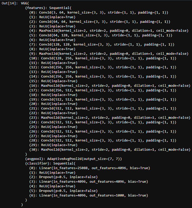
After initializing the VGG-16 model for transfer learning, the output layer must be updated to reflect the scenario. In this case, from 1000 neurons to 2 (one for dog and the other for cat). You must send the layer to the GPU device otherwise there will be feed-forward and backpropagation.
model.classifier[-1] = nn.Linear(in_features=4096, out_features= 2).to(device)
def train(model, train_dl, val_dl, num_epochs):


    criterion = nn.CrossEntropyLoss()
    # Observe that all parameters are being optimized
    optimizer = optim.SGD(model.parameters(), lr=0.001, momentum=0.9)
    # Decay LR by a factor of 0.1 every 7 epochs
    scheduler = optim.lr_scheduler.StepLR(optimizer, step_size=7, gamma=0.1)

    val_accuracies = []
    train_accuracies = []

    # Repeat for each epoch
    for epoch in range(num_epochs):
        running_loss = 0.0
        correct_prediction = 0
        total_prediction = 0

        # Repeat for each batch in the training set
        for i, data in enumerate(train_dl):
            # Get the input features and target labels, and put them on the GPU

            inputs, labels = data[0].to(device), data[1].to(device)

            # Zero the parameter gradients
            optimizer.zero_grad()

            # forward + backward + optimize
            outputs = model(inputs)
            loss = criterion(outputs, labels)
            loss.backward()
            optimizer.step()
            scheduler.step()

            # Keep stats for Loss and Accuracy
            running_loss += loss.item()

            # Get the predicted class with the highest score
            _, prediction = torch.max(outputs,1)

            # Count of predictions that matched the target label
            correct_prediction += (prediction == labels).sum().item()
            total_prediction += prediction.shape[0]

            # if i % 10 == 0:    # print every 10 mini-batches
                # print('[%d, %5d] loss: %.3f' % (epoch + 1, i + 1, running_loss / 10))

        # Print stats at the end of the epoch
        num_batches = len(train_dl)
        avg_loss = running_loss / num_batches
        acc = correct_prediction/total_prediction

        # Run Model against Validation Set
        val_acc = inference(model, val_dl)
        val_accuracies.append( (epoch, val_acc))
        train_accuracies.append( (epoch, acc))

        print(f'Epoch: {epoch}, Loss: {avg_loss:.2f}, Training Accuracy: {acc:.2f}, Validation Accuracy: {val_acc:.2f}')

    return val_accuracies, train_accuracies
For each epoch, run mini-batches from the data loader into the neural network. After making predictions, compare against the training data and calculate the differences via CrossEntropyLoss function. Make the gradient adjustment via backpropagation and report accuracy and validation accuracy.
val_accuracies, train_accuracies = train(model, train_dl,val_dl, num_epochs = 3)
After one epoch, the neural network can accurately predict images at 94% training and 96% validation accuracy. Additional epochs did not make a significant difference in accuracy. If we set weights = False, then we would expect additional epochs.
def make_predictions (model, test_dl):
     # Disable gradient updates
    file_names = []
    predictions = []
    with torch.no_grad():
        for data in test_dl:
            # Get the input features and target labels, and put them on the GPU

            inputs, paths = data[0].to(device), data[1]


            for path in paths:
                file_name = path.split('/')[-1]
                file_names.append(file_name)

            # Normalize the inputs
            inputs_m, inputs_s = inputs.mean(), inputs.std()
            inputs = (inputs - inputs_m) / inputs_s

            # Get predictions
            outputs = model(inputs)

            # Get the predicted class with the highest score
            _, prediction = torch.max(outputs,1)


            for i, x in enumerate(prediction):
                predictions.append(x.item())

            # print(prediction)

    return file_names, predictions
file_names, predictions = make_predictions(model, test_dl)

test_predictions_df = pd.DataFrame(list(zip(file_names, predictions)),
           columns =['file_name', 'predicted_class_id'])
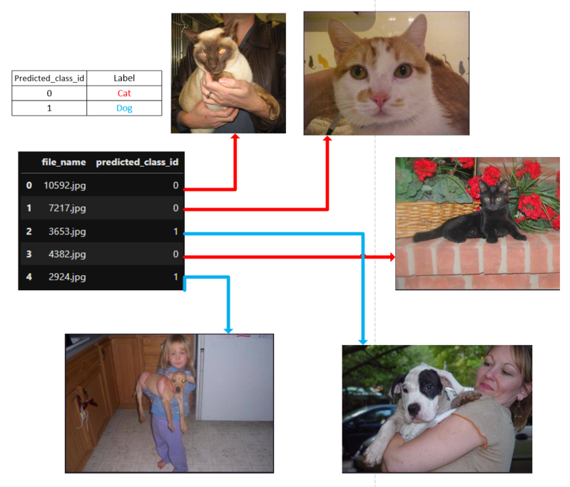
Alternatively, if using script mode, create an endpoint using model artifacts generated from completed training:
model = Model(image_uri=container,
              model_data=model_url,
              role=role)

model.deploy(
    initial_instance_count=1,
    instance_type="ml.g4dn.xlarge",
    endpoint_name=endpoint_config_name
)